See previous post on Big O Notation: Time Flies with Big O Notation: Improving Algorithm Efficiency - Part 1.

Let's get right to it.

In this series, we'll talk about O(n log n), O(n^2), O(2^n), and O(n!).

Big O notation visualized (again)

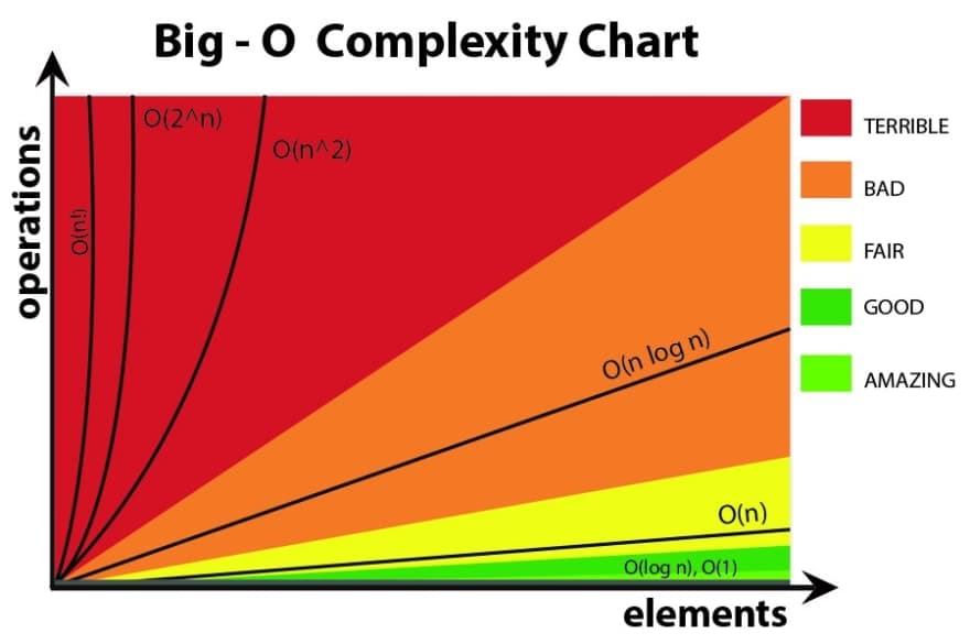
O(n log n) - The Efficient Middle Ground

O(n log n) is commonly seen in efficient sorting algorithms like Merge Sort and Quick Sort. Here, the input size 'n' grows, and for each element, there’s a logarithmic growth of operations.

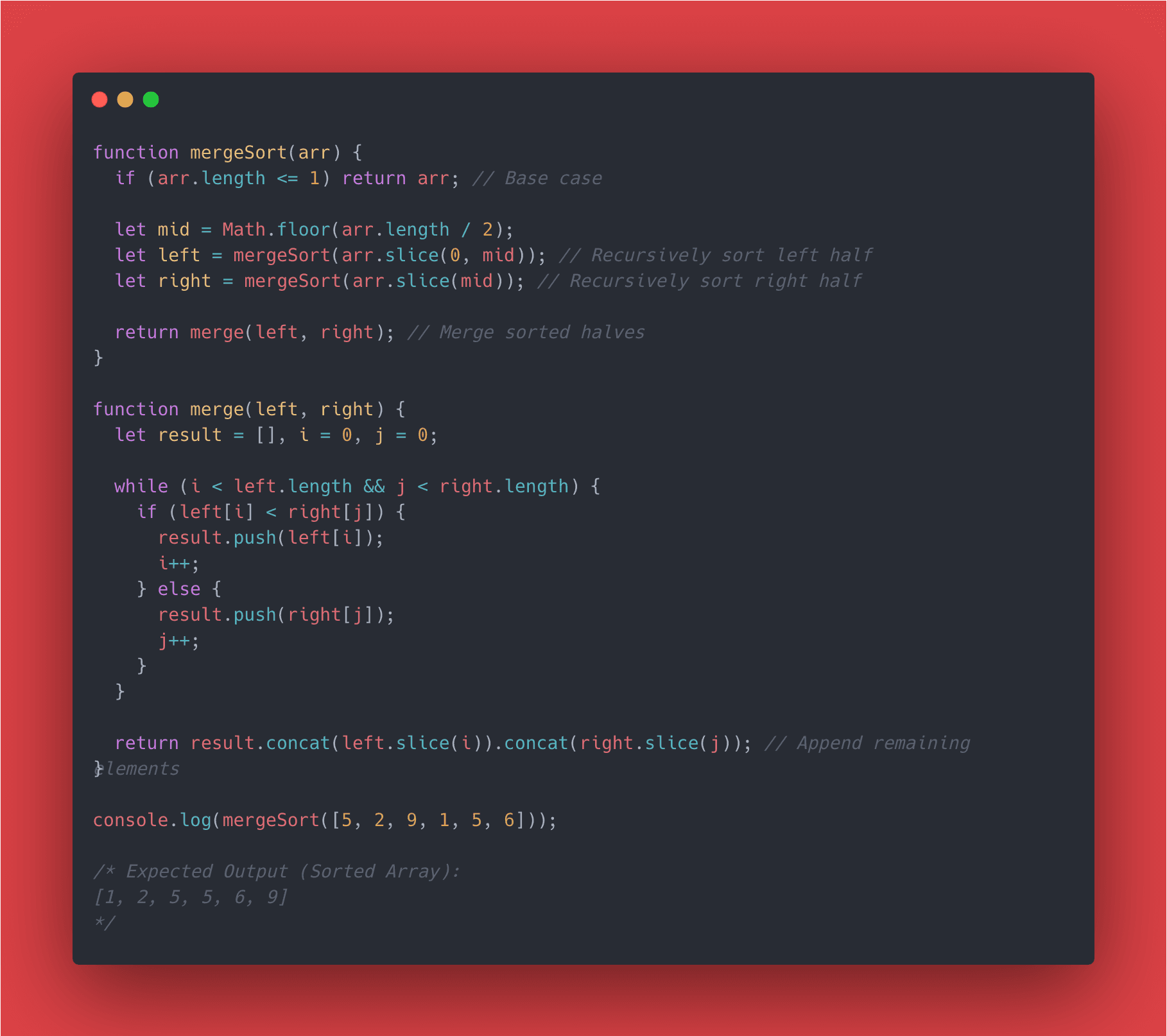
An algorithm that represents O(n log n) is a merge sort. Merge Sort algorithm splits an array in half recursively until each half contains a single element, and then merges them back together in sorted order. The splitting part happens in O(log n) time, and the merging part happens in O(n) time for each level of recursion. Let's look at a merge sort algorithm.

O(n²) - The Classic Quadratic Complexity

O(n²) represents algorithms where the time it takes to run grows quadratically as the input size increases. This is often seen in algorithms that involve nested loops, where for each element, the algorithm must iterate over the entire dataset again. Let’s look at Bubble Sort, a straightforward but inefficient sorting algorithm.

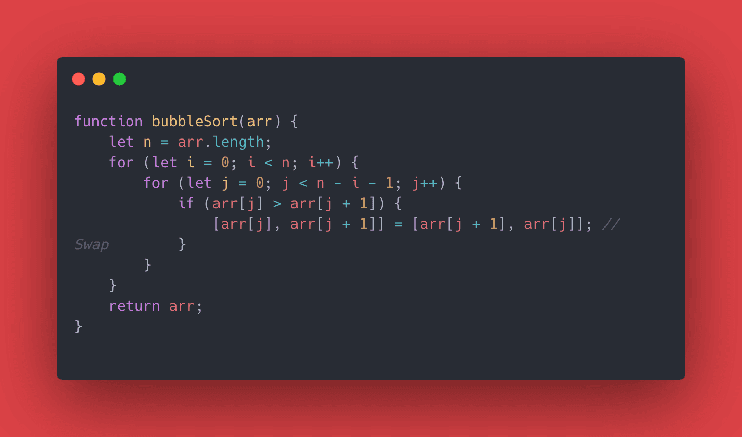
Here, the outer loop runs 'n' times, and for each iteration of the outer loop, the inner loop runs 'n-i-1' times. This gives us an overall time complexity of O(n²). As you can imagine, for large datasets, this quickly becomes inefficient, which is why O(n log n) algorithms are generally preferred for sorting.

O(2ⁿ) - The Exponential Explosion

O(2^n) describes algorithms where the runtime doubles with each additional element in the input set. This often appears in problems involving combinations, permutations, or recursive solutions where each call branches into two more calls. Consider a naive recursive solution to the Fibonacci sequence, where each number is the sum of the two preceding ones.

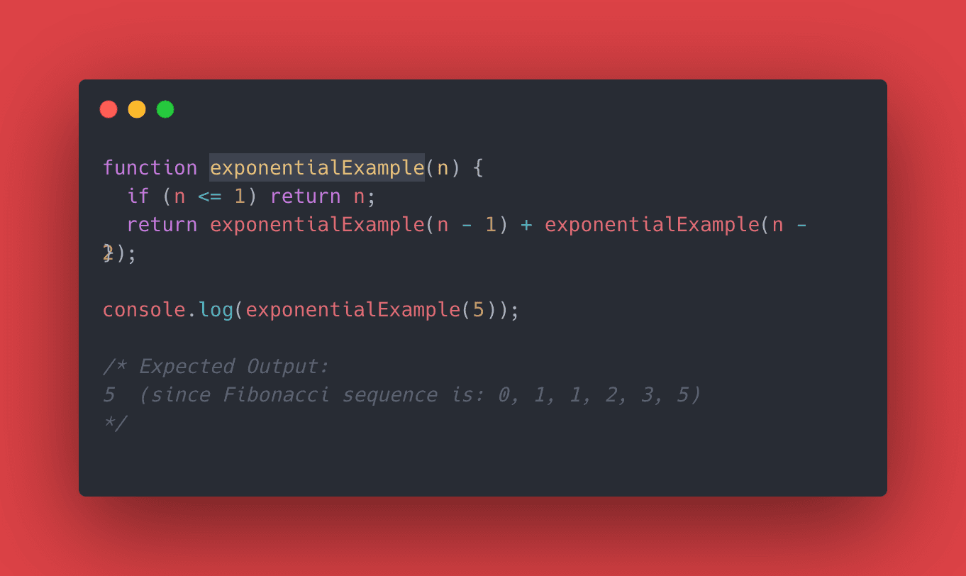
In this example, fibonacci(5) calculates fibonacci(4) and fibonacci(3), each of which further branches into multiple recursive calls. The number of calls grows exponentially, leading to a time complexity of O(2^n). For small inputs, this might be fine, but it quickly becomes impractical as 'n' grows larger.

O(n!) - The Factorial Nightmare

O(n!) represents algorithms where the time required to complete the task grows factorially with the size of the input. These are the most complex and least efficient algorithms, often seen in brute-force approaches to problems like the Traveling Salesman Problem, where every possible permutation of paths is explored. Imagine generating all permutations of a list of numbers.

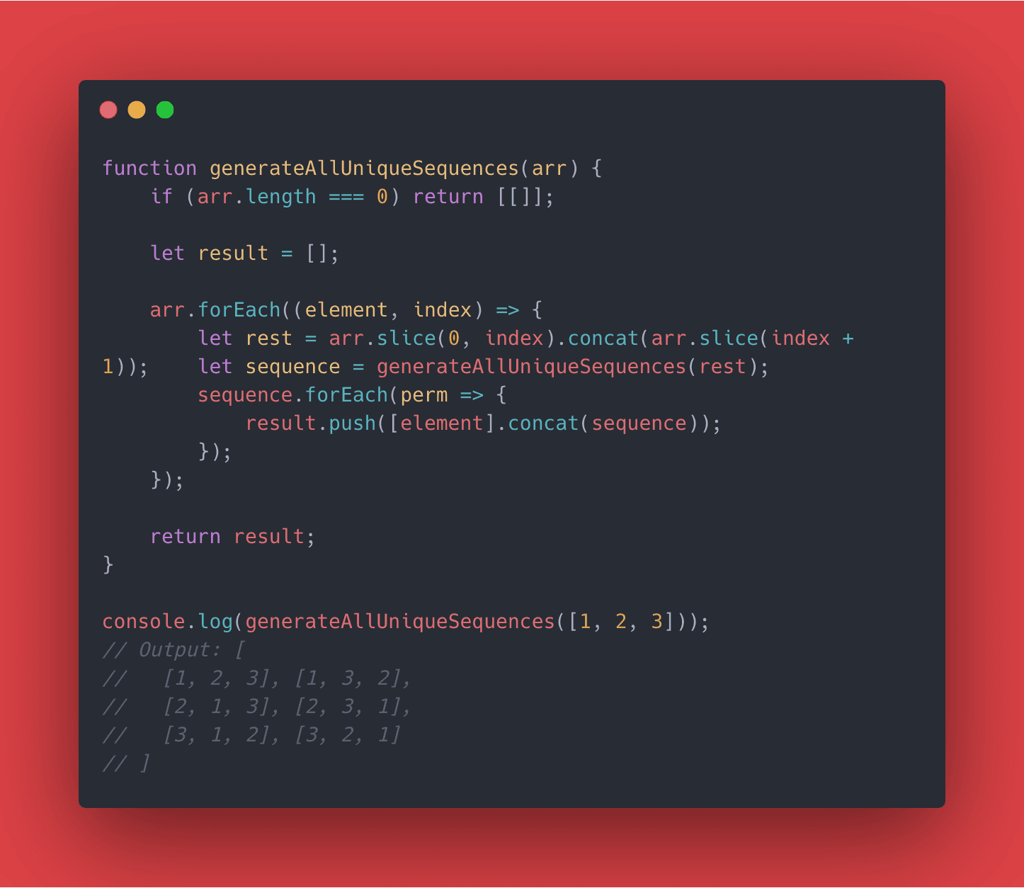
For an input list of length 'n', there are n! (n factorial) possible permutations. So, as 'n' increases, the number of permutations—and thus the time required—grows extraordinarily fast. This makes O(n!) algorithms only feasible for very small datasets.

Wrapping Up: Choosing the Right Algorithm

Understanding Big O Notation is like having a superpower that lets you see the future of your code’s performance. For junior developers, this knowledge is invaluable because it helps you make informed decisions about which algorithms to use and when to use them. Always remember that while O(n log n) is often the sweet spot for sorting algorithms, sometimes the simplicity of O(n^2) is all you need. However, beware of the exponential and factorial time complexities (O(2^n) and O(n!))—these can quickly make your algorithms impractical for large inputs.

When you're choosing an algorithm, consider the size of your input data and how critical performance is for your application. With practice, recognizing and applying Big O Notation will become second nature, helping you write code that not only works but works efficiently.

Until next time, Happy Computing!!

RO out 🎤